Candlestick chart patterns: read the prices before the pattern
Reconstruct open, high, low, and close, understand fill conventions, and distinguish a descriptive candle pattern from a prediction.
Read the guideWork through a five-session simple moving average, warm-up values, smoothing, lag, and the settings a useful legend should preserve.
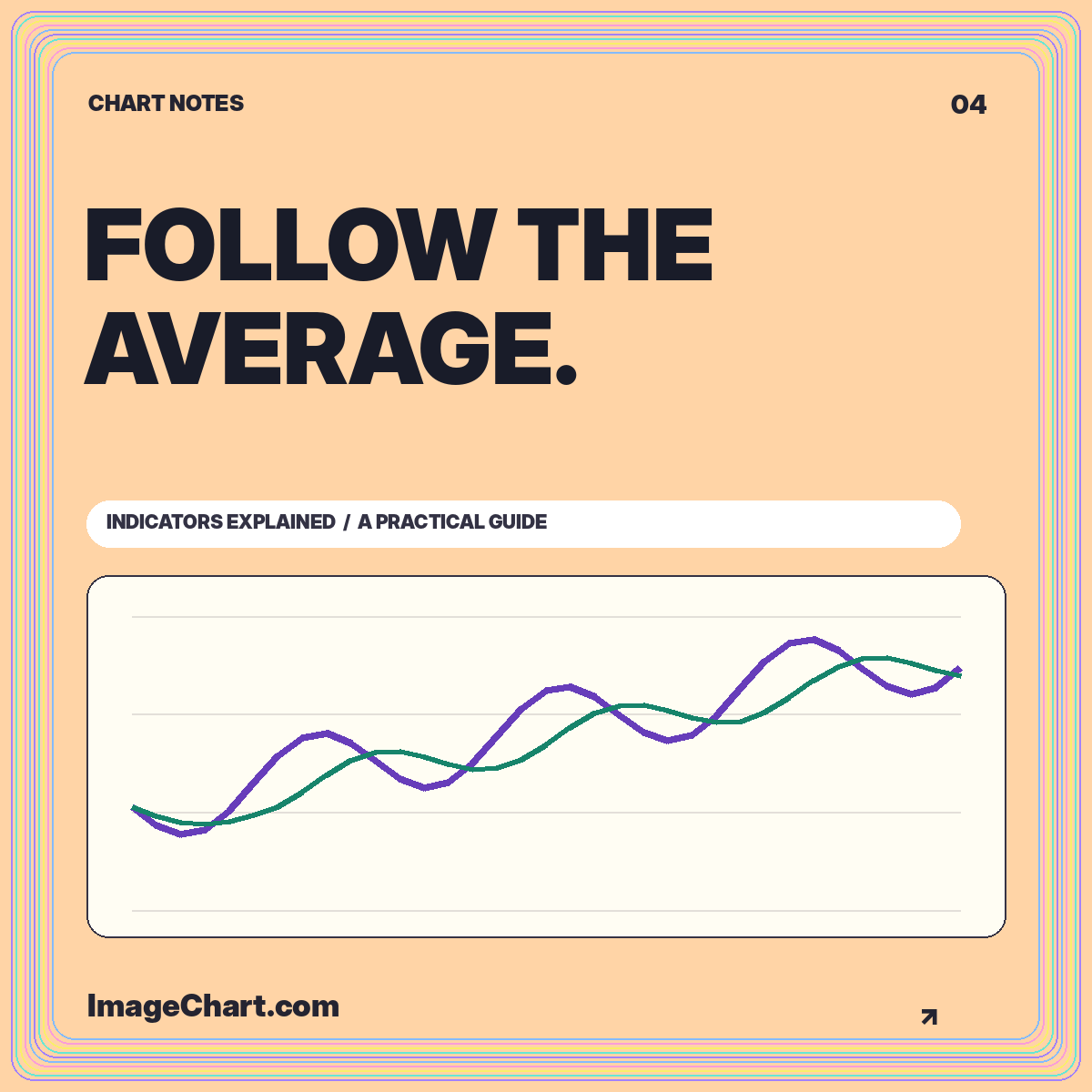
A moving average is easy to add to a chart and surprisingly easy to mislabel. The line depends on the averaging method, the number of observations, the sampling interval, and the input field. Omitting any of these details makes the chart harder to reproduce and can change what a reader thinks the line represents.
This guide works through a simple moving average using invented closing values. The aim is to explain the calculation and its visual tradeoffs, not to turn a crossover into investment advice. You can examine a five-session average in the trend and average template or toggle it in the chart studio.
A five-period simple moving average takes five selected observations, adds them, and divides the sum by five. Fidelity’s simple moving average explanation describes this equal-weight calculation. “Period” refers to the chart’s input interval; it does not automatically mean a calendar day.
If the values are daily session closes, five periods means five such observations. If they are weekly closes, the same window length spans five weekly observations. Missing dates and non-trading days make it especially important to describe the input sequence rather than loosely calling every average a daily measure.
A useful legend might say “5-session SMA of closing index.” That tells readers the count, method, and field. The chart subtitle can then identify the sampling interval, source, and adjustment treatment. These small labels are more informative than a legend that says only “MA.”
Take five invented closing values: 100, 102, 101, 105, and 107. Their sum is 515, so the first five-observation average is 103. Plot that value at the fifth observation when using a trailing average. The calculation summarizes the current and preceding four observations; it does not belong at the center of the window.
Now add a sixth close of 110. The oldest value, 100, leaves the window and 110 enters. The new sum is 525, giving an average of 105. Notice that the current close rose three units, from 107 to 110, while the average rose two. The line’s movement reflects the replacement of an old observation, not simply the latest price change.
A compact table is an excellent companion to this example. Show the observation number, close, and average where available. Readers can check the arithmetic without estimating line positions on an image. Exact values and visual trends support different reading tasks.
With a five-observation window, the first four positions do not yet have a complete trailing average. Leave those values unavailable unless you explicitly choose a different initialization convention. Inserting zeros would create a false plunge. Averaging shorter windows would produce a changing definition that needs to be disclosed.
The ImageChart example leaves the first four average values blank. Once the full synthetic history has been calculated, a shorter displayed window can still show average values based partly on observations just outside the crop. This is appropriate when the caption explains that the indicator was calculated from the full available sequence before display filtering.
Do not recalculate the first visible average from only the cropped points unless that is the intended methodology. Otherwise, changing the zoom level can change the computed indicator rather than merely changing its visible range. That is a substantive difference, not a harmless presentation preference.
An average suppresses some variation by combining observations. It can make a general direction easier to inspect, but it also conceals the exact path within the window. Different sequences can share the same mean. A flat average therefore does not prove that the underlying observations were stable.
For example, the values 98, 99, 100, 101, and 102 average to 100. So do 90, 110, 95, 105, and 100. The center is the same, but the second sequence varies more. Showing the average without the original line would erase a distinction that may matter to the explanation.
Keep the unsmoothed series visible when teaching the relationship. Use a restrained overlay color or a dashed line for the average, and give it a direct label. A larger lookback usually produces a visually smoother historical summary, but the specific appearance still depends on the data.
A trailing average incorporates earlier observations, so its response depends on the entire current window. When the original series changes direction, older values remain in the calculation until they leave the window. That is a consequence of the definition, not an implementation mistake.
Consider a series that holds at 100 for several observations and then moves to 120. The first five-period average containing one 120 and four 100s is 104. It reaches 120 only after the window contains five values of 120. The average’s gradual rise is an arithmetic result of the rolling composition.
Whether this is useful depends on the question. A smoothed historical overview may be easier to communicate than every small fluctuation. A task requiring the latest observation should not substitute the average for that current value. Put both measures in the caption when their difference is central to the story.
A simple moving average assigns equal weight to the observations inside its defined window. An exponential average uses a recursive weighting scheme that gives newer observations different influence. Its exact result depends on the smoothing parameter and initialization convention. Naming only a period count is not enough to guarantee identical values across implementations.
For a reproducible educational graphic, document the formula or reference the chosen implementation. Do not silently switch averaging methods between screenshots while keeping the same legend. Readers may otherwise attribute differences to the data when they actually arise from a different transformation.
A side-by-side comparison should share the same input series, interval, and display scale. Explain the purpose of comparing methods rather than declaring one universally better. The useful question is which summary suits the task and what information it hides, not which line looks closest to a later turning point.
When two lines cross, that geometric relationship is visible and describable. For example, a close can move above its trailing average, or a shorter-window average can move above a longer-window average. Neither event alone establishes what happens next or whether a particular trade would be suitable.
Avoid selecting a dramatic historical crossover after seeing the subsequent outcome and labeling it a proven signal. A chart can demonstrate the definition while remaining neutral about predictive value. Evaluating a rule requires a broader, explicitly defined process than illustrating one attractive example.
The technical analysis chart guide explains the distinction between descriptive indicators and strategy testing. In a publishing context, the most useful crossover annotation identifies the relevant observation and states exactly which lines changed relative position. It should not add a profit claim that the image cannot support.
Include the method, lookback, input field, interval, and warm-up treatment in the graphic or adjacent description. If the visible history is shorter than the calculation history, say so. An exported image should not lose those definitions when it leaves the interactive interface.
Check contrast and line patterns at the final viewing size. The average should remain distinguishable from the original series in a narrow mobile card or a grayscale printout. Do not use a decorative glow that blurs the point where the line crosses a reference level. A clear stroke with an explicit legend is easier to inspect.
Keep enough significant figures for verification without implying unnecessary precision. The table may show two decimals while the main axis uses whole units. That is a display choice, not a reason to calculate the average from previously rounded chart labels.
A well-designed moving-average chart helps readers connect a formula with its visual effect. They should be able to identify the input series, reconstruct a sample value, and understand why the smoothed line differs from the latest observation. Those are concrete, teachable outcomes.
Use smoothing to clarify a historical relationship, not to make uncertainty disappear. The best overlay leaves its assumptions visible and gives the original observations room to remain part of the story. When the arithmetic, labels, and visual hierarchy agree, a simple chart can explain a great deal.
All worked numerical examples are hypothetical. Educational material, not personal investment advice. See our data and editorial methodology.
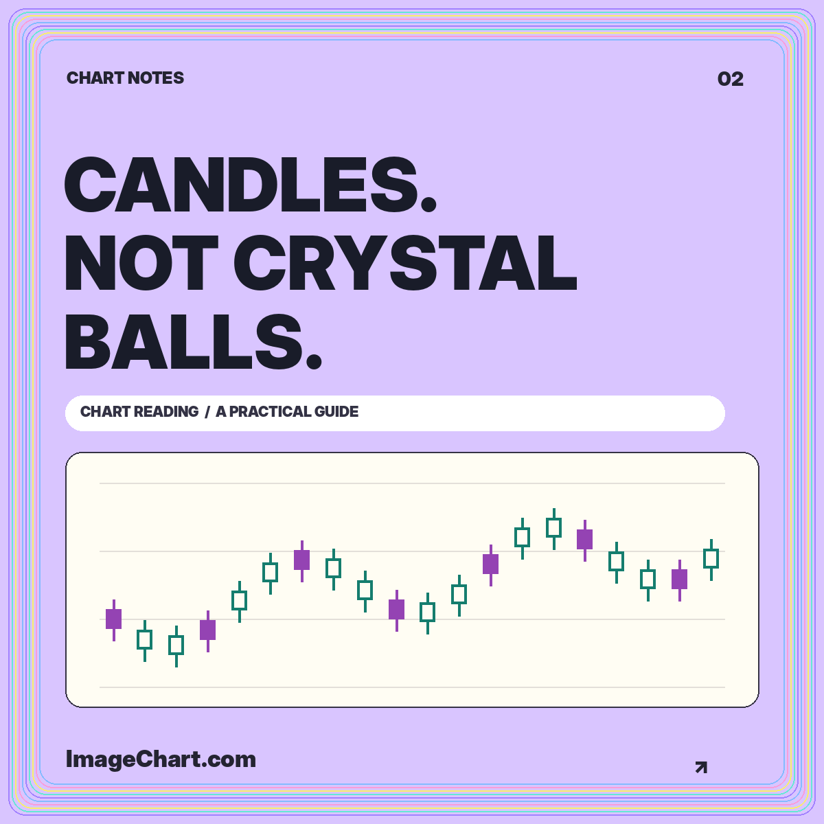
Reconstruct open, high, low, and close, understand fill conventions, and distinguish a descriptive candle pattern from a prediction.
Read the guide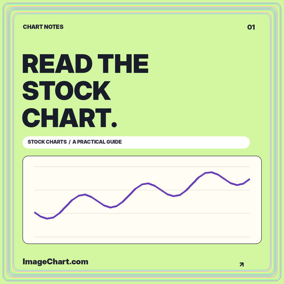
Learn a repeatable approach to chart identity, intervals, scales, price changes, and the difference between a visible pattern and an explanation.
Read the guide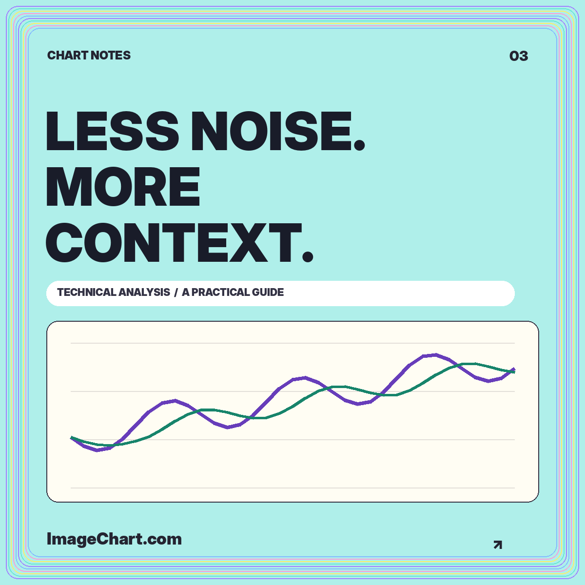
Give overlays, volume, and momentum measures separate jobs, document the settings, and keep historical summaries distinct from forecasts.
Read the guide